5. GridPath Functionality - High Level
In this chapter, we discuss GridPath’s functionality at a high level. It is subdivided into three sections:
5.1. Approaches
GridPath can be used in production-cost simulation or capacity-expansion mode depending on whether “projects” of the “new” capacity types are included in the model.
5.1.1. Production-Cost Simulation
Production-cost simulation models, also called unit-commitment and dispatch models, simulate the operations of a specified power system with a high level of fidelity – at a high temporal resolution (e.g. hours to 5-minute segments) and considering the detailed operating characteristics of generators – but generally over a fairly short period of time (e.g. optimizing a year one day at a time). These models are adept at optimizing the day-to-day operations of a fixed electric power system, provide information on system reliability, assess transmission congestion, and produce simulated locational marginal prices. They can also be used to evaluate the impact of additions or retirements of capacity. As the number of resources under considerations increases, however, so does the number of possible combinations we need to simulate, making analysis using production-cost simulation increasingly intensive and cumbersome. Answering questions about how to develop the grid in the future as demand, technologies, and policies change therefore requires additional types of modeling capability.
5.1.2. Capacity-Expansion
While production cost simulation models seek to optimize the operations of a power system with a fixed set of resources specified by the user, capacity-expansion models are designed to understand how the system should evolve over time: they try to answer the question of what resources to invest in among many options in order to meet system goals over time, i.e. what grid infrastructure is most cost-effective while ensuring that the system operates reliably and meeting policy targets.
The capacity expansion model minimizes the overall system cost over some planning horizon, considering both capital costs (generators, transmission, storage, any asset) and variable or operating costs subject to various technical (e.g. generator limits, wind and solar availability, transmission limits across corridors, hydro limits) and policy constraints (e.g. renewable energy mandates, GHG targets).
Because capacity-expansion models have to optimize over several years or decades, selecting generation, and transmission assets from many different available options, the problem can get large quickly. In order to have reasonable runtime, these models often simplify aspects of the electricity grid, both in space and time. Spatially, most models will consider only balancing areas or states as nodes (so all substations with the BA are clubbed together). Temporally, only representative days and hours may be used, and then given weights to represent a whole year e.g. one day per month, and either 24 hours, or 6 time blocks (each representing 4 hours). This simplification makes the linear optimization problem tractable. If the spatial resolution is small, the temporal resolution may be increased, and vice versa. An advantage of GridPath is that, unlike other similar platforms, it leaves the decision for where to simplify and where to add resolution to the user, making it possible to tailor the problem formulation to the question at hand, the available computational resources, and the available time.
After the system is “built” by a capacity-expansion problem, the system may be simulated for the entire year (or years) using the production-cost functionality to ensure that the decisions made using representative time slices produce a system that can operate reliably at every time point of the year. Capacity-expansion and production cost models are therefore complementary. The former allows us to quickly explore many options for how the power system ought to evolve over time and find the optimal solution; the latter can help us ensure that the system we design does in fact perform as we intended (e.g. that it serves load reliably and meets policy targets).
GridPath’s architecture makes it possible for the same modules to be re-used in production-cost or capacity-expansion modeling setting, allowing for a seamless transition from one approach to the other, as datasets can be more easily shared and reused.
5.1.3. Asset-Valuation
GridPath can include market functionality and can optimize the dispatch of a resource or a set of resources to maximize market revenue while meeting other system constraints.
5.1.4. Resource Adequacy
GridPath can be used to evaluate the system’s resource adequacy, e.g., by using dispatch modeling over many load, renewable output, and generator and transmission outage conditions.
5.1.5. Linear, Mixed-Integer, and Non-Linear Formulations
Depending on how modules are combined, linear, mixed-integer, and non-linear problem formulations are possible in GridPath. Some modules are interchangeable, with the variable domain (e.g. binary vs. continuous with 0 to 1 bounds) the only difference in the final formulation.
5.2. Basic Functionality
GridPath can be used to create optimization problems with different features and varying levels of complexity. For the basic model, the user must define:
Temporal Setup : The model’s temporal setup (e.g. 365 individual days at an hourly resolution),
Geographic Setup : The geographic setup (e.g. a single load zone),
Projects : The availability and operating characteristics of the generation infrastructure (e.g. an existing 500-MW coal plant with a specified heat rate),
Objective Function : The desired objective (e.g. minimize cost).
5.2.1. Temporal Setup
GridPath’s temporal span and resolution are flexible: the user can decide on a temporal setup by assigning appropriate weights to and relationships among GridPath’s temporal units.
The temporal units include:
Timepoints
Timepoints are the finest resolution over which operational decisions are made (e.g. an hour). Generator commitment and dispatch decisions are made for each timepoint, with some constraints applied across timepoints (e.g. ramp constraints.) Most commonly, a timepoint is an hour, but the resolution is flexible: a timepoint could also be a 15-minute, 5-minute, 1-minute, or 4-hour segment. Different timepoint durations can also be mixed, e.g. some can be 5-minute segments and some can be hours.
Timepoints can also be assigned weights in order to represent other timepoints that are not modeled explicitly (e.g. use a 24-hour period per month to represent the whole month using the number of days in that month for the weight of each of the 24 timepoints). Note that all costs incurred at the timepoint level are multiplied by the period-level number_years_represented and discount_factor parameters in the objective function. At the period level we use annualized capacity costs (and multiply those by the number of years in a period), so we must also annualize operational costs incurred at the timepoint level. In other words, we must use the timepoint weights (along with the hours-in-timepoint parameter) to calculate the timepoint-level cost incurred over a year. The sum of timepoint_weight*hours_in_timepoint over all timepoints in a period must therefore equal the number of hours in a year (8760, 8766, or 8784). This will then get multiplied by the number of years in a period and period discount rate to get the total operational costs.
For example, if you are representing a 10-year period with a single day at a 24-hour timepoint resolution, the timepoint weight for each of the 24 timepoints would need to be 365. Timepoint-level costs will be multiplied by 10 automatically to account for the length of the period. If you are representing a 1-year period with a single day at a 24-hour resolution, the timepoint weight would still be 365, and timepoint-level costs will get multiplied by 1 automatically to account for the length of the period. If you are representing a 0.25-year period with a single day at a 24-hour resolution, the timepoint weight would still be 365.
To support multi-stage production simulation timepoints can also be assigned a mapping to the previous stage (e.g. timepoints 1-12 in the 5-minute real-time stage map to timepoint 1 in the hour-ahead stage) and a flag whether the timepoint is part of a spinup or lookahead segment.
Timepoints that are part of a spinup or lookahead segment are included in the optimization but are generally discarded when calculating result metrics such as annual emissions, energy, or cost.
See Subproblems and Stages for more information.
Balancing Types and Horizons
GridPath organizes timepoints into balancing types and horizons that describe how timepoints are grouped together when making operational decisions, with some operational constraints enforced over the horizon for each balancing type, e.g. hydro budgets or storage energy balance. As a simple example, in the case of modeling a full year with 8760 timepoints, we could have three balancing types: a day, a month, and a year; there would then be 365 horizons of the balancing type ‘day,’ 12 horizons of the balancing type ‘month,’ and 1 horizon of the balancing type ‘year.’ Within each balancing types, horizons are modeled as independent from each other for operational purposes (i.e operational decisions made on one horizon do not affect those made on another horizon). Generator and storage resources in GridPath are also assigned balancing types: a hydro plant of the balancing type ‘day’ would have to meet an energy budget constraint on each of the 365 ‘day’ horizons whereas one of the balancing type ‘year’ would only have a single energy budget constraint grouping all 8760 timepoints.
Each horizon has boundary condition that can be ‘circular,’ ‘linear,’ or ‘linked.’ With the ‘circular’ approach, the last timepoint of the horizon is considered the previous timepoint for the first timepoint of the horizon (for the purposes of functionality such as ramp constraints or tracking storage state of charge). If the boundary is ‘linear,’ then we ignore constraints relating to the previous timepoint in the first timepoint of a horizon. If the boundary is ‘linked,’ then we use the last timepoint of the previous horizon as the previous timepoint for the first timepoint of a horizon (this can only be done when running multiple subproblems and inputs must be specified appropriately).
Periods
Each timepoint in a GridPath model also belongs to a period (e.g. a year), which describes when decisions to build or retire infrastructure are made. A period must be specified in both capacity-expansion and production-cost models. In a production-cost simulation context, we can use the period to exogenously change the amount of available capacity, but the period temporal unit is mostly used in the capacity-expansion approach, as it defines when capacity decisions are made and new infrastructure becomes available (or is retired). That information in turn feeds into the horizon- and timepoint-level operational constraints, i.e. once a generator is build, the optimization is allowed to operate it in subsequent periods (usually for the duration of the generators’s lifetime). You must specify period duration via the period_start_year and period_end_year parameters (the duration is calculated within GridPath based on those values). Note that the start year is inclusive and the end year is exclusive. Capacity can either exist or not for the entire duration of a period. A discount factor can also be applied to weight costs differently depending on when (in which period) they are incurred.
Warning
Support for investment periods that are shorter than 1 year, e.g. monthly investment decisions, is largely untested, so be extra careful if attempting to use this functionality.
Subproblems
In production-cost simulation, we often model operations during a full year, e.g. at an hourly resolution (8760 timepoints). However, not all timepoints are optimized together. Usually, each day or week of the year is optimized separately. In GridPath, these separate optimizations are called subproblems. Each subproblem can then contain different balancing types and horizons. For example, if we are optimizing the year’s operations a week at a time, we would have 52 subproblems. Each one of those subproblems could then have two balancing types – a week and a day – meaning each timepoint in the subproblem would belong to one of seven ‘day’ horizons and the single ‘week’ horizon (i.e. some resources would have to be balanced on each day of the week and some over the entire week).
Within a production-cost simulation subproblem, some timepoints can be part of a spin-up or look-ahead segment. These are additional timepoints that are added to the subproblem’s start and end but are ultimately discarded when calculating result metrics. They are there to more faithfully model the beginning and start of the subproblem. For example, if we had weekly subproblems we could add 24 hourly spinup timepoins (1 day) before the week, and 24 hourly lookahead timepoints (1 day) after the week, resulting in 52 subproblems of 9 days. After solving each subproblem independently, the 2 edge days in each subproblem are discarded .
Unlike in production-cost simulation, in capacity-expansion mode, we usually have only a single subproblem (and no spinup or lookahead timepoints).
Stages
GridPath also has multi-stage commitment functionality, i.e. commitment decisions made for a subproblem can be fixed and then fed into a next stage with some updated parameters (e.g. an updated load and renewable output forecast). The number of stages is flexible and the timepoint resolution can change from stage to stage.
For instance, the same day (subproblem) could first be modeled using a day-ahead hourly forecast (“DA stage”), then with an hour-ahead hourly forecast (“HA stage”), and finally with a real-time 5-minute forecast (“RT stage”). Commitment decisions for e.g. coal generators could be fixed in the DA stage, whereas commitment for e.g. gas turbines could be changed until the final RT stage.
In practice, this is achieved by assigning a stage to each timepoint and specifying a map between timepoints in each stage (see Timepoints). Load and renewable forecast inputs are indexed by timepoint and stage, allowing for different forecasts (and, optionally, timepoint resolutions) in each stage.
Examples
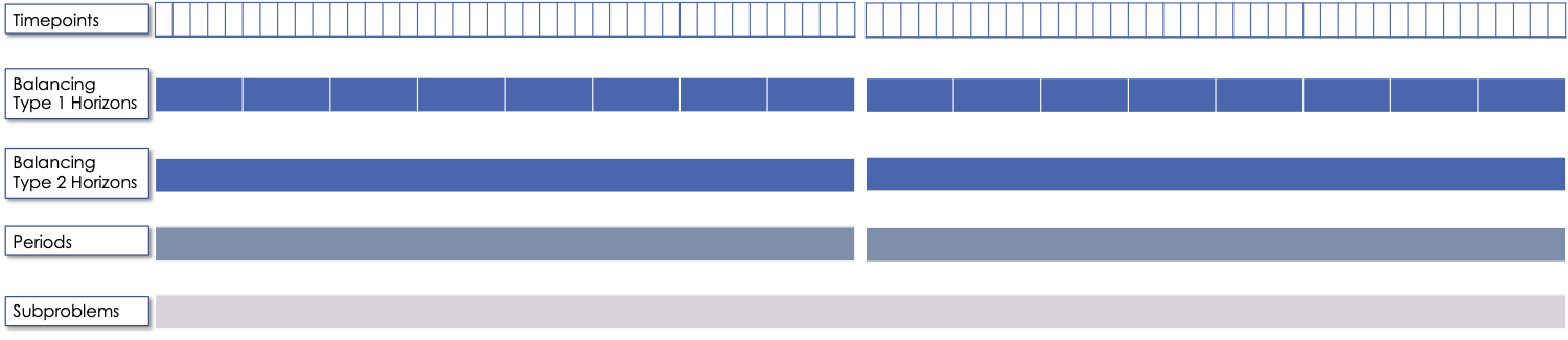
A typical temporal setup for capacity-expansion modeling is shown below. Note the presence op multiple investment periods, and a single subproblem and stage (i.e. a single optimization).
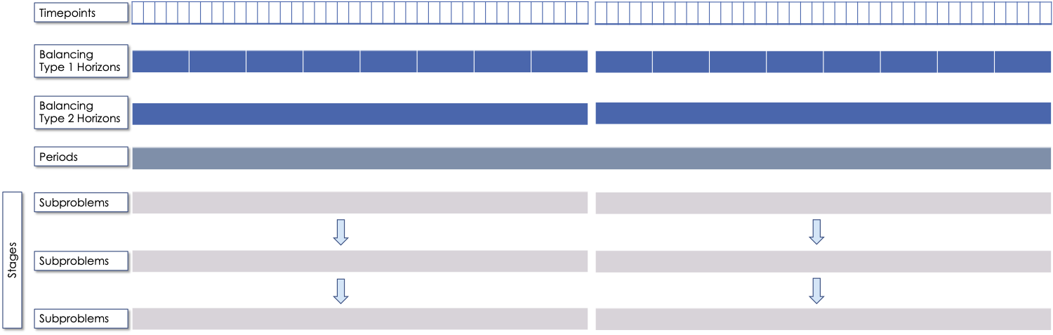
A typical temporal setup for production-cost modeling is shown below. Note the presence of a single period, and multiple subproblems and stages (i.e. an optimization will be solved for every subproblem-stage combination).
5.2.2. Geographic Setup
Load Zones
The main geographic unit in GridPath is the load zone. The load zone is the level at which the load-balance constraints are enforced. In GridPath, we can model a single load zone (copper plate) or multiple load zones, which can be connected with transmission. This flexibility makes it possible to apply to different regions with different geographic set-up or to take different geographic approaches in modeling the same region (e.g. higher or lower zonal resolution for the same region).
Other Geographic Units
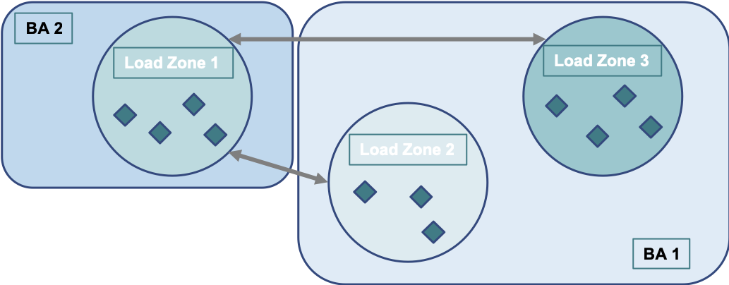
Optional levels of geographic resolution include balancing areas (BAs) for operational and reliability reserve requirements and policy zones for policy requirements. In GridPath, it is possible for generators in the same load zone to contribute to different reserve balancing areas and/or policy zones. Two possible configurations are shown below.
Geographic Configuration 1:
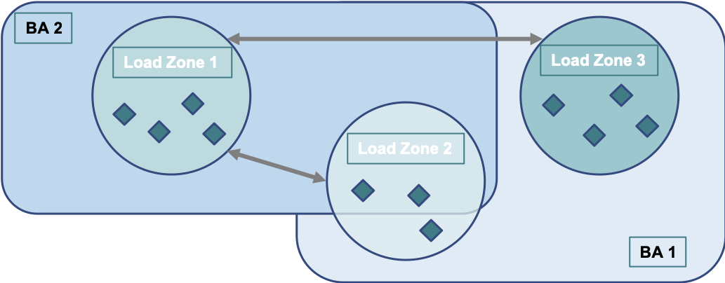
Geographic Configuration 2:
5.2.3. Projects
Generation, storage, and load-side resources in GridPath are called projects. Each project is associated with a load zone whose load-balance constraint it contributes to. In addition, each project must be assigned a capacity type, an availability type, and an operational type. These types are described in more detail below.
Project Capacity Types
Each project in GridPath must be assigned a capacity type. The capacity type determines the capacity and the capacity-associated costs of generation, storage, and demand-side infrastructure projects in the optimization problem. The currently implemented capacity types include:
Specified Generation (gen_spec)
This capacity type describes generator projects that are available to the optimization without having to incur an investment cost, e.g. existing projects or projects that will be built in the future and whose capital costs we want to ignore (in the objective function). A specified generator can be available at a specified capacity in all periods, or in some periods only, with no restriction on the order and combination of periods or the variation in capacity by period.
The user may specify a fixed O&M cost for these generators, but this cost will be a fixed number in the objective function and will therefore not affect any of the optimization decisions.
Specified Generation with Linear Economic Retirement (gen_ret_lin)
This capacity type describes generator projects with the same characteristics as gen_spec, but whose fixed O&M cost can be avoided by ‘retiring’ them.
The optimization can make the decision to retire generation in each study period. Once retired, the generator may not become operational again. Retirement decisions for this capacity type are ‘linearized,’ i.e. the optimization may retire generators partially (e.g. retire only 200 MW of a 500-MW generator). If retired, the annual fixed O&M cost of these projects is avoided in the objective function.
Specified Generation with Binary Economic Retirement (gen_ret_bin)
This capacity type describes generators with the same characteristics as gen_ret_lin. However, retirement decisions are binary, i.e. the generator is either fully retired or not retired at all.
Linear New-Build Generation (gen_new_lin)
This capacity type describes new generation projects that can be built by the optimization at a cost. These investment decisions are linearized, i.e. the decision is not whether to build a unit of a specific size (e.g. a 50-MW combustion turbine), but how much capacity to build at a particular project. Once built, the capacity remains operational and fixed O&M costs are incurred for the duration of the project’s pre-specified operational lifetime. Minimum and maximum capacity constraints can be optionally implemented.
The capital cost input to the model is an annualized cost per unit capacity. If the optimization makes the decision to build new capacity, the total annualized cost is incurred in each period of the study (and multiplied by the number of years the period represents) for the duration of the project’s financial lifetime.
Binary New-Build Generation (gen_new_bin)
This capacity type describes new generation projects that can be built by the optimization at a pre-specified size and cost. The model can decide to build the project at the specified size in some or all investment periods, or not at all. Once built, the capacity remains operational and fixed O&M costs are incurred for the duration of the project’s pre-specified operational lifetime.
The capital cost input to the model is an annualized cost per unit capacity. If the optimization makes the decision to build new capacity, the total annualized cost is incurred in each period of the study (and multiplied by the number of years the period represents) for the duration of the project’s financial lifetime.
Specified Storage (stor_spec)
This capacity type describes the power (i.e. charging and discharging capacity) and energy capacity (i.e., duration – see important note on interaction with discharge efficiency) of storage projects that are available to the optimization without having to incur an investment cost. For example, it can be applied to existing storage projects or to storage projects that will be built in the future and whose capital costs we want to ignore (in the objective function).
It is not required to specify a capacity for all periods, i.e. a project can be operational in some periods but not in others with no restriction on the order and combination of periods. The user may specify a fixed O&M cost for specified-storage projects, but this cost will be a fixed number in the objective function and will therefore not affect any of the optimization decisions.
Note
Please note that to calculate the duration of the storage project, i.e., how long it can sustain discharging at its maximum output, you must adjust the energy capacity by the discharge efficiency. For example, a 1 MW with 1 MWh energy capacity battery with discharging losses of 5% (discharging_loss_factor = 95%) would have a duration of 1 MWh / (1 MW/0.95) or 0.95 hours rather than 1 hour.
Linear New-Build Storage (stor_new_lin)
This capacity type describes storage projects that can be built by the optimization at a cost. Investment decisions are made separately for the project’s power capacity and its energy capacity, therefore endogenously determining the duration sizing of the storage. The decisions are linearized, i.e. the model decides how much power capacity and how much energy capacity to build at a project, not whether or not to build a project of pre-defined capacity. Once built, the capacity remains operational and fixed O&M costs are incurred for the duration of the project’s pre-specified operational lifetime. Minimum and maximum power capacity and duration constraints can be optionally implemented.
The capital cost input to the model is an annualized cost per unit of power capacity (MW) and an annualized cost per unit energy capacity (MWh). The costs are additive. If the optimization makes the decision to build new power/energy capacity, the total annualized cost is incurred in each period of the study (and multiplied by the number of years the period represents) for the duration of the project’s financial lifetime.
Note
Please note that to calculate the duration of the storage project, i.e., how long it can sustain discharging at its maximum output, you must adjust the energy capacity by the discharge efficiency. For example, a 1 MW with 1 MWh energy capacity battery with discharging losses of 5% (discharging_loss_factor = 95%) would have a duration of 1 MWh / (1 MW/0.95) or 0.95 hours rather than 1 hour.
Binary New-Build Storage (stor_new_bin)
This capacity type describes new storage projects that can be built by the optimization at a pre-specified size, duration and cost. The model can decide to build the project at the specified size in some or all investment periods, or not at all. Once built, the capacity remains operational and fixed O&M costs are incurred for the duration of the project’s pre-specified operational lifetime.
The capital cost input to the model is an annualized cost per unit of power capacity (MW) and an annualized cost per unit energy capacity (MWh). The costs are additive. If the optimization makes the decision to build new power/energy capacity, the total annualized cost is incurred in each period of the study (and multiplied by the number of years the period represents) for the duration of the project’s financial lifetime.
Note
Please note that to calculate the duration of the storage project, i.e., how long it can sustain discharging at its maximum output, you must adjust the energy capacity by the discharge efficiency. For example, a 1 MW with 1 MWh energy capacity battery with discharging losses of 5% (discharging_loss_factor = 95%) would have a duration of 1 MWh / (1 MW/0.95) or 0.95 hours rather than 1 hour.
Specified Generation-Storage Hybrid (gen_stor_hyb_spec)
This capacity type describes generator-storage hybrid projects that are “specified,” i.e. available to the optimization without having to incur an investment cost. We specify grid-facing capacity as well as the capacity of the generator component and the power and energy capacity of the storage component. Each of those is associated with a fixed cost.
Shiftable Load Supply Curve (dr_new)
This type is a custom implementation for GridPath projects in the California Integrated Resource Planning proceeding (2018ish). It is outdated.
This capacity type describes a supply curve for new shiftable load (DR; demand response) capacity. The supply curve does not have vintages, i.e. there are no cost differences for capacity built in different periods. The cost for new capacity is specified via a piecewise linear function of new capacity build and constraint (cost is constrained to be greater than or equal to the function).
The new capacity build variable has units of MWh. We then calculate the power capacity based on the ‘minimum duration’ specified for the project, e.g. if the minimum duration specified is N hours, then the MW capacity will be the new build in MWh divided by N (the MWh capacity can’t be discharged in less than N hours, as the max power constraint will bind).
Specified Fuel Production Facilities (fuel_prod_spec)
This capacity type describes fuel production facilities with exogenously specified capacity characteristics.
Note that it is usually the case that you also need to enforce fuel burn limits to ensure that only fuel produced by projects of this type (and potentially ‘fuel_prod_new’) can be used by other projects.
Candidate Fuel Production Facilities (fuel_prod_new)
This capacity type describes fuel production projects that can be built by the optimization at a cost. Investment decisions are made separately for the project’s fuel production, fuel release, and fuel storage capacity, therefore endogenously determining the sizing of the facility. The decisions are linearized.
Like with new-build generation, capacity costs added to the objective function include the annualized capital cost and the annual fixed O&M cost.
Project Availability Types
Each project in GridPath must be assigned an availability type that determines how much of a project’s capacity is available to operate in each timepoint. For example, some or all of a project’s capacity may be unavailable due to maintenance and other planned or unplanned outages. The following availability types have been implemented.
Exogenous
For each project assigned this availability type, the user may specify an (un)availability schedule, i.e. a capacity derate for each timepoint in which the project may be operated. If fully derated in a given timepoint, the available project capacity will be 0 in that timepoint and all operational decision variables will therefore also be constrained to 0 in the optimization.
Binary
Projects assigned this availability type have binary decision variables for their availability in each timepoint. This type can be useful in optimizing planned outage schedules. A project of this type is constrained to be unavailable for at least a pre-specified number of hours in each period. In addition, each unavailability event can be constrained to be within a minimum and maximum number of hours, and constraints can also be implemented on the minimum and maximum duration between unavailability events.
Continuous
This availability type is formulated like the binary type except that all binary decision variables are relaxed to be continuous with bounds between 0 and 1. This can be useful to address computational difficulties when modeling endogenous project availabilities.
Project Operational Types
Each project in GridPath must be assigned an operational type. The operational_type determines the operational capabilities of a project. The currently implemented operational types include:
Simple Generation (gen_simple)
This operational type describes generators that can vary their output between zero and full capacity in every timepoint in which they are available (i.e. they have a power output variable but no commitment variables associated with them).
The heat rate of these generators does not degrade below full load and they can be allowed to provide upward and/or downward reserves subject to available headroom and footroom. Ramp limits can be optionally specified.
Costs for this operational type include fuel costs, variable O&M costs, and startup and shutdown costs.
Must-Run Generation (gen_must_run)
This operational type describes must-run generators that produce constant power equal to their capacity in all timepoints when they are available.
The available capacity can either be a set input (e.g. for the gen_spec capacity_type) or a decision variable by period (e.g. for the gen_new_lin capacity_type). This makes this operational type suitable for both production simulation type problems and capacity expansion problems.
The heat rate is assumed to be constant and this operational type cannot provide reserves (since there is no operable range, i.e. no headroom or footroom).
Costs for this operational type include fuel costs and variable O&M costs.
Always-On Generation (gen_always_on)
This module describes the operations of generation projects that that must produce power in all timepoints they are available; unlike the must-run generators, however, they can vary power output between a pre-specified minimum stable level (greater than 0) and their available capacity.
The available capacity can either be a set input (e.g. for the gen_spec capacity_type) or a decision variable by period (e.g. for the gen_new_lin capacity_type). This makes this operational type suitable for both production simulation type problems and capacity expansion problems.
The optimization makes the dispatch decisions in every timepoint. Heat rate degradation below full load is considered. Always-on projects can be allowed to provide upward and/or downward reserves, subject to the available headroom and footroom. Ramp limits can be optionally specified.
Costs for this operational type include fuel costs and variable O&M costs.
Binary-Commit Generation (gen_commit_bin)
This operational types describes generation projects that can be turned on and off, i.e. that have binary commitment variables associated with them. This is particularly useful for production cost modeling approaches where capturing the unit commitment decisions is important, e.g. when modeling a slow-starting coal plant. This operational type is not compatible with new-build capacity types (e.g. gen_new_lin) where the available capacity is an endogenous decision variable.
The optimization makes commitment and power output decisions in every timepoint. If the project is not committed (or starting up / shutting down), power output is zero. If it is committed, power output can vary between a pre-specified minimum stable level (greater than zero) and the project’s available capacity. Heat rate degradation below full load is considered. These projects can be allowed to provide upward and/or downward reserves.
Startup and/or shutdown trajectories can be optionally modeled by specifying a low startup and/or shutdown ramp rate. Ramp rate limits as well us minimum up and down time constraints are implemented. Starts and stops – and the associated cost and emissions – can be tracked and constrained.
Costs for this operational type include fuel costs, variable O&M costs, and startup and shutdown costs.
Interesting background papers: - “Hidden power system inflexibilities imposed by traditional unit commitment formulations”, Morales-Espana et al. (2017). - “Tight and compact MILP formulation for the thermal unit commitment problem”, Morales-Espana et al. (2013).
Continuous-Commit Generation (gen_commit_lin)
This operational type is the same as the gen_commit_bin operational type, but the commitment decisions are declared as continuous (with bounds of 0 to 1) instead of binary, so ‘partial’ generators can be committed. This linear relaxation treatment can be helpful in situations when mixed-integer problem run-times are long and is similar to loosening the MIP gap (but can target specific generators). Please refer to the gen_commit_bin module for more information on the formulation.
Capacity-Commit Generation (gen_commit_cap)
This module describes the operations of generation projects with ‘capacity commitment’ operational decisions, i.e. continuous variables to commit some level of capacity below the total capacity of the project. This operational type is particularly well suited for application to ‘fleets’ of generators with the same characteristics. For example, we could have a GridPath project with a total capacity of 2000 MW, which actually consists of four 500-MW units. The optimization decides how much total capacity to commit (i.e. turn on), e.g. if 2000 MW are committed, then four generators (x 500 MW) are on and if 500 MW are committed, then one generator is on, etc.
The capacity commitment decision variables are continuous. This approach makes it possible to reduce problem size by grouping similar generators together and linearizing the commitment decisions.
The optimization makes the capacity-commitment and dispatch decisions in every timepoint. Project power output can vary between a minimum loading level (specified as a fraction of committed capacity) and the committed capacity in each timepoint when the project is available. Heat rate degradation below full load is considered. These projects can be allowed to provide upward and/or downward reserves.
No standard approach exists for applying ramp rate and minimum up and down time constraints to this operational type. GridPath does include experimental functionality for doing so. Starts and stops – and the associated cost and emissions – can also be tracked and constrained for this operational type.
Costs for this operational type include fuel costs, variable O&M costs, and startup and shutdown costs.
Curtailable Hydro Generation (gen_hydro)
This operational type describes the operations of hydro generation projects. These projects can vary power output between a minimum and maximum level specified for each horizon, and must produce a pre-specified amount of energy on each horizon when they are available, some of which may be curtailed. Negative output is allowed, i.e. this module can be used to model pumping. The curtailable hydro projects can be allowed to provide upward and/or downward reserves. Ramp rate limits can optionally be enforced.
Costs for this operational type include variable O&M costs.
Non-Curtailable Hydro Generation (gen_hydro_must_take)
This operational type describes the operations of hydro generation projects and is like the gen_hydro operational type except that the power output is must-take, i.e. curtailment is not allowed. Negative output is allowed, i.e. this module can be used to model pumping.
Curtailable Variable Generation (gen_var)
This operational type describes generator projects whose power output is equal to a pre-specified fraction of their available capacity (a capacity factor parameter) in every timepoint, e.g. a wind farm with variable output depending on local weather. Curtailment (dispatch down) is allowed. GridPath includes experimental features to allow these generators to provide upward and/or downward reserves.
Costs for this operational type include variable O&M costs.
Non-curtailable Variable Generation (gen_var_must_take)
This operational type is like the gen_var type with two main differences. First, the project’s output is must-take, i.e. curtailment (dispatch down) is not allowed. Second, because the project’s output is not controllable, projects of this operational type cannot provide operational reserves .
Storage (stor)
This operational type describes a generic storage resource. It can be applied to a battery, to a pumped-hydro project or another storage technology.
The type is associated with three main variables in each timepoint when the project is available: the charging level, the discharging level, and the energy available in storage. The first two are constrained to be less than or equal to the project’s power capacity. The third is constrained to be less than or equal to the project’s energy capacity. The model tracks the stage of charge in each timepoint based on the charging and discharging decisions in the previous timepoint, with adjustments for charging and discharging efficiencies. Storage projects can be allowed to provide upward and/or downward reserves.
Costs for this operational type include variable O&M costs.
Note
Please note that to calculate the duration of the storage project, i.e., how long it can sustain discharging at its maximum output, you must adjust the energy capacity by the discharge efficiency. For example, a 1 MW with 1 MWh energy capacity battery with discharging losses of 5% (discharging_loss_factor = 95%) would have a duration of 1 MWh / (1 MW/0.95) or 0.95 hours rather than 1 hour.
Note
Model construction performance: most components in this module are indexed by project-timepoint, so their initialization and constraint/ expression rules are called once per index – millions of times in production-scale scenarios. Per-index work that only depends on the project (or can be looked up once) is therefore deliberately hoisted:
STOR_OPR_BT_HRZchecks horizon-timepoint membership element-by-element with O(1) lookups againstPRJ_OPR_TMPSand iterates only the project’s own balancing type’s horizons. (Testing withset(...).issubset(mod.PRJ_OPR_TMPS)would materialize the entire multi-million-element superset into a temporary Python set on every check.)The reserve expressions delegate to
gridpath.project.operations.reserves.reserve_aggregation, which resolves reserve variable names to component objects once per model instance instead of callinggetattrper index.The tracking/ramp-style rules look up
mod.balancing_type_project[prj]andmod.prev_tmp[...]once per call and reuse the local, rather than re-indexing the params for every term of the returned expression.Derived sets initialized by filtering a superset do not re-declare that superset as
within– the domain check is redundant with the initializer and roughly doubles set construction time. (Sets loaded from input data, likeSTOR_EXOG_SOC_TMPS, keepwithinsince there it validates user input.)
Curtailable Variable Generation-Storage Hybrid (gen_var_stor_hyb)
This operational type describes a tightly-coupled variable resource and storage hybrid project, e.g. solar and battery hybrid project where the battery can only charge from the solar component and not from the grid, and the total power output of the project from the solar and battery components is limited separately from each individual component.
We track power availability from the variable resource via a capacity factor parameter and the amount of power that goes directly to the grid and the amount that is stored. The former is limited by the power capacity of the generator component and the latter by the charging power capacity of the battery. The model tracks the state of charge of the battery. Total grid power output from the project (from the generator component and from storage discharging) is limited by the project’s nameplate capacity. This operational type can also be curtailed, and can provide both upward and downward reserves.
Costs for this operational type include variable O&M costs and, optionally, a cost on curtailment.
Warning
This module has not been extensively used and vetted, so be extra vigilant for buggy behavior.
Flexible Load (flex_load)
This operational type describes a battery-based model for a flexible load resource. Please use gen_spec as the ‘capacity type’ for flexible loads.
Note that a previous module (dr) for flexible loads is now deprecated.
Fuel Production (fuel_prod)
This operational type describes the operational constraints on fuel production facilities.
The type is associated with three main variables in each timepoint when the project is available: the fuel production level, the fuel release level, and the fuel available in storage. The first two are constrained to be less than or equal to the project’s fuel production and fuel release capacity respectively. The third is constrained to be less than or equal to the project’s fuel storage capacity. The model tracks the amount of fuel available in storage in each timepoint based on the fuel production and fuel release decisions in the previous timepoint. Fuel production projects do not provide reserves or other system services.
Costs for this operational type include variable O&M costs, currently based on the project’s power consumption (note that this is applied through the generic variable_om_cost_per_mwh parameter, which is specified in project.operatons.__init__.
Note that it is usually the case that you also need to enforce fuel burn limits to ensure that only fuel produced by projects of this type can be used by other projects.
Dispatchable Load (dispatchable_load)
This operational type describes dispatchable loads. Their “power output” is subtracted from the power-production side of the load-balance constraints.
Projects of this type may have a heat rate associated with them, for example to model direct air capture facilities that consume power in order to capture carbon from the atmosphere. Note that this should be modeled to burn a fuel with a negative emissions intensity and they do require a simple heat rate. Also note that projects of this type must be assigned a carbon cap zone in order to contribute net negative emissions to the carbon constraint.
Project of this type may have a consumption ratio associated with them, for example synchornous condenser consumes 1%-3% of their nameplate capacity in order to operate and produce inertia.
5.2.4. Load Balance
The load-balance constraint in GridPath consists of production components and consumption components that are added by various GridPath modules depending on the selected features. The sum of the production components must equal the sum of the consumption components in each zone and timepoint.
At a minimum, for each load zone and timepoint, the user must specify a static load requirement input as a consumption component. On the production side, the model aggregates the power output of projects in the respective load zone and timepoint.
Note
Net power output from storage and demand-side resources can be negative and is currently aggregated with the ‘project’ production component.
Net transmission into/out of the load zone is another possible production component (see Transmission).
The user may also optionally allow unserved energy and/or overgeneration to be incurred by adding the respective variables to the production and consumption components respectively, and assigning a per unit cost for each load-balance violation type.
5.2.5. Objective Function
GridPath’s objective function consists of modularized components. This modularity allows for different objective functions to be defined. Here, we discuss the objective of maximizing the net present value of revenues minus costs.
Its most basic version includes the aggregated project capacity costs and aggregated project operational costs, and any load-balance penalties incurred (i.e. the aggregated unserved energy and/or overgeneration costs).
Other standard objective function components include:
aggregated transmission line capacity investment costs
aggregated transmission operational costs (hurdle rates)
aggregated reserve violation penalties
GridPath also can include custom objective function components that may not be standard for all systems. Examples currently include:
local capacity shortage penalties
planning reserve margin costs
various tuning costs
Market costs and revenues may also be included.
GridPath can include costs on carbon emissions, so certain formulations can interpreted as minimizing emissions.
All revenue and costs are in net present value terms, with a user-specified discount factor applied depending on the period.
5.3. Optional Functionality
GridPath contains a number of modules that are optional. These modules are:
Transmission : to model tranmission flows between multiple load zones,
Operating Reserves : to model reserves such as frequency regulation or spinning reserves,
Markets : to model policy measures such as a Renewable Portfolio Standard (RPS) or a carbon cap,
Reliability: to model system reliability through a planning reserve marging (PRM) constraint, and
Custom Modules : GridPath’s modularity allows for easy addition of custom constraints specific to a power grid.
5.3.1. Transmission
In GridPath, the user can include transmission line flows and transmission topography by selecting the ‘transmission’ feature and specifying the available transmission lines and which load zones they connect.
For each load zone and timepoint, the net flow on all transmission lines connected to the load zone is aggregated and added as a production component to the load balance constraint (see Load Balance).
Note
If there is a net flow out of a load zone, the load-balance constraint ‘production’ component is a negative number.
Transmission features modules also add a transmission-capacity-costs component and a transmission-operational-costs component to the objective function (see Objective Function).
Like with GridPath ‘projects,’ transmission lines must be assigned a capacity type, which determines their capacity and costs, and an operational type, which determines their operational characteristics and costs.
The transmission network in GridPath can currently be modeled using a linear transport model or using DC power flow (see Transmission Operational Types). In either approach, resistive losses are assumed to be negligible.
Transmission Capacity Types
Each transmission line in GridPath must be assigned a capacity type. The line’s capacity type determines the available transmission capacity and the capacity-associated costs. The currently implemented capacity types include:
Specified Transmission (tx_spec)
This capacity type describes transmission lines that are available to the optimization without having to incur an investment cost, e.g. existing lines or lines that will be built in the future and whose capital costs we want to ignore (in the objective function). A specified transmission line can be available in all periods, or in some periods only, with no restriction on the order and combination of periods. The two transmission line directions may have different specified capacities, e.g. a line from Zone 1 to Zone 2 with a minimum flow capacity of -1,000 MW and a maximum flow capacity of 1,200 MW can transmit up to 1,000 MW from Zone 2 to Zone 1 and up to 1,200 MW from Zone 1 to Zone 2.
Linear New-Build Transmission (tx_new_lin)
This capacity type describes transmission lines that can be built by the optimization at a cost. These investment decisions are linearized, i.e. the decision is not whether to build a specific transmission line, but how much capacity to build at a particular transmission corridor. Once built, the capacity remains available for the duration of the line’s pre-specified lifetime. The line flow limits are assumed to be the same in each direction, e.g. a 500 MW line from Zone 1 to Zone 2 will allow flows of 500 MW from Zone 1 to Zone 2 and vice versa.
The cost input to the model is an annualized cost per unit capacity. If the optimization makes the decision to build new capacity, the total annualized cost is incurred in each period of the study (and multiplied by the number of years the period represents) for the duration of the transmission line’s lifetime.
Transmission Operational Types
Transmission lines in GridPath must be assigned an operational type. The operational type determines the formulation of the operational capabilities of the transmission line. The operational types currently implemented include:
Linear Transport Transmission (tx_simple)
This operational type describes transmission lines whose flows are simulated using a linear transport model, i.e. transmission flow is constrained to be less than or equal to the line capacity. Line capacity can be defined for both transmission flow directions. The user can define losses as a fraction of line flow.
DC Power Flow (tx_dcopf)
This operational type describes transmission lines whose flows are simulated using DC optimal power flow (OPF) equations. DC power flow is a linearized approach to the AC Optimal Power Flow problem, which is a non-linear, non-convex set of equations describing the energy flow through each transmission line. The three main assumptions for the DC power flow approximation are:
line resistances are negligible compared to line reactances, so reactive power flows can be neglected;
voltage magnitudes at each bus are kept at their nominal value; and
voltage angle differences across branches are small enough such that the sine of the difference can be approximated by the difference, i.e. \(\sin(\\theta) \\approx \\theta\).
Using these approximations, the power flow problem becomes linear and can be added to our capacity-expansion / unit commitment model using an additional set of constraints for flows on each tx_dcopf line. The DC OPF constraints are based on the Kirchhoff approach laid out in “Horsch et al. (2018). Linear Optimal Power Flow Using Cycle Flows”.
Warning
Transmission operational types can be optionally be mixed. However, if there are any transmission lines that do not have the tx_dcopf operational types, they will simply not be considered when setting up the network constraints laid out in the tx_dcopf module, so the network flows will be inaccurate.
Warning
GridPath uses one user-specified reactance to characterize a transmission line and this value doesn’t change across time periods, even when the planned transmission capacity changes or when the model selects to build additional capacity (in the case of new build transmission). If this is not a reasonable assumption for the transmission system of interest, we recommended not to use the tx_dcopf operational type.
5.3.2. Operating Reserves
GridPath can optionally model a range of operating reserve types, including regulation up and down, spinning reserves, load-following up and down, inertia reserves and frequency response. The implementation of each reserve type is standardized. The user must define the reserve balancing areas along with any penalties for violation of the reserve-balance constraints. For each balancing area, the reserve requirement for each timepoint must be specified. Only exogenously-specified reserves are implemented at this stage. Each project that can provide the reserve type must then be assigned a balancing area to whose reserve-balance constraint it can contribute. The project-level reserve-provision variables are dynamically added to the project’s operating constraints if the project can provide each reserve type. Total reserve provision by projects in each balancing area is then aggregated and constrained to equal the BA’s reserve requirement in each timepoint. The user can optionally allow these constraints to be violated at a cost. Any reserve-balance constraint violation penalty costs are added to the objective function.
5.3.3. Reliability
GridPath can optionally model a planning-reserve margin requirement (PRM). The user must the define the zones with a PRM requirement and the requirement level for each PRM zone and period. Each project that can contribute capacity (i.e. expected load-carrying capability – ELCC – greater than 0) must be assigned a PRM zone to whose reserve-balance constraint it can contribute. The PRM reserve-balance constraint is a period-level constraint. Projects can contribute a fraction of their capacity as their ELCC via the prm_simple module. See Custom Modules) for some advanced reliability functionality.
5.3.4. Markets
GridPath can allow a resource or a set of resources to participate in markets with pre-specified price streams, assuming resources are price-takers and subject to market volume limits.
5.3.5. Policy
Energy Targets (e.g., Renewable Portfolio Standard)
GridPath can optionally impose targests for energy production by eligible projects, e.g., renewable portfolio standard (RPS) requirements. The user must first define the zones with an RPS requirement. The RPS requirement is a period- or horizon-level constraint. Each RPS-eligible project must be assigned an RPS zone to whose requirement it can contribute. The amount of RPS-eligible energy a project contributes in each timepoint is determined by its operational type (e.g. a must-run biomass plant will contribute its full capacity times the timepoint duration in every timepoint while a wind project will contribute its capacity factor times its capacity). The model aggregates all projects’ contributions for each period and ensures that the RPS requirement is met in each RPS zone and period.
Instantaneous Penetration
GridPath can optionally impose minimal and maximal constraints on the instantaneous penetration of eligible projects. The user must first define the zones with instantaneous penetration requirements. The instantaneous penetration requirement is a timepoint constraint. Each instantaneous penetration-eligible project must be assigned an instantaneous penetration zone, and the model aggregates all projects contributions for each timepoint ensuring that the total penetration respects the set minimum and maximum requirement. The minimum and maximum penetration requirements are set as the sum of:
Exogenously input power levels (MW) at a timepoint resolution.
A percentage of the load at every timepoint.
The capacity of other projects.
The Power output of other projects.
As a default, all requirements are set at 0 except for the percentage of the load for the maximum penetration which is set to 100%.
Carbon Cap or Carbon Cost
GridPath can optionally impose an carbon cap constraint. The user must first define the zones with an emissions cap and the cap level by period (not all periods must have a requirement). Each carbon-emitting project must be assigned a carbon cap zone to whose emissions it can contribute. The amount of carbon emissions from a project in each timepoint is determined by its operational type and fuel. The model aggregates all projects’ contributions for each period and ensures that the total emissions stay below the cap in each carbon cap zone and period.
GridPath can also optionally apply an emissions factor to energy imports into an emissions zone. For the purpose, the relevant transmission lines (i.e. transmission lines that connect the emissions zone to other zones) must be assigned an emissions zone and an emissions intensity per unit energy. These emissions are then added to the emissions cap constraint.
The emissions cap could be applied to carbon emissions or to other types of emissions.
Alternatively, GridPath can model a cost on carbon emissions and optimize the amount of emissions.
Fuel Use Limits
GridPath can be used to impose constraints on the amount of fuel available to generators over certain time periods.
Performance Standard
GridPath can optionally impose a performance standard requirement, i.e. limiting the emissions intensity of energy produced by a set of projects.
5.3.6. Custom Modules
GridPath can include custom modules depending on the region or system models. For example, for studies in the California Integrated Resource Planning proceedings, GridPath includes constraints on transmission simultaneous flow limits and advanced reliability functionality such as:
ELCC surface module: this module has substantial exogenous data requirements, but makes it possible to dynamically adjust the ELCC of some projects depending on the resource build-out (e.g. as more solar is built, the marginal ELCC becomes smaller)
Energy-only / partial deliverability: ability to de-rate ELCC eligibility to less than the full project capacity (before applying the simple PRM fraction or the ELCC surface), since in some cases full deliverability may require additional costs to be incurred (e.g. for transmission, etc.)
Energy-limits: additional limits on ELCC based on energy-limitations (e.g. for storage)
Similar custom functionality can be added for other systems and easily excluded when not needed.